Announcements
Please also check Canvas for class announcements.
Week 14 Announcement
In the last week we will explore Monte Carlo methods — a powerful numerical approach to evaluate high dimensional integrals that relies on random numbers. Monte Carlo approaches can be used to sample from any kind of distributions and are therefore suitable to directly simulate physical systems according to the Boltzmann distribution, which underpins statistical mechanics of, for example, simple models of magnetism.
Week 10-12 Announcement
For the next three weeks we will learn how to solve partial differential equations (PDEs). PDEs underpin all manner of physical phenomena, as soon as a quantity depends on more than one independent variable. Commonly the independent variables are the three dimensions of space and time. Unlike ordinary differential equations, there’s no “one size fits all” approach. For different types of equations we will need different algorithms. We start with problems in electrostatic (Poisson’s equation), move to diffusion and heat conduction problems (diffusion equation), and close with wave problems (wave equation).
Your Final Project is also about to start, so we will have discussions about the project and your project pitches where you will form your project teams around your project proposals.
Week 9 Announcement
A lot of physics can be formulated in the language of linear algebra with vectors and matrices. Examples are problems in solid body mechanics and quantum mechanics. Three commonly encountered requirements are to find solutions to a matrix equation \(\mathsf{A} \mathbf{x} = \mathbf{b}\), finding the inverse of a matrix \(\mathsf{A}^{-1}\), and solving the eigenproblem \(\mathsf{A} \mathbf{v}_i = \lambda_i \mathbf{v}_i\). Instead of writing our own solvers, we will learn how to use the routines in numpy.linalg, NumPy’s linear algebra module, which provides efficient and well-tested algorithm.
A matrix solver is also needed for generalizing the Newton-Raphson root finding algorithm from the last module to arbitrary dimensions. We will develop a general Newton-Raphson solver (and also learn how to calculate the Jacobian using partial derivatives, based on the central difference algorithm from the lesson on differentiation).
Week 8.5 Announcement
A common problem is to find the roots \(x_0\) of an equation, \(f(x_0)=0\). We will develop two algorithms to find roots numerically. The bisection algorithm is a simple and robust approach that exemplifies how to go from imagining a solution (“how would I solve this problem?”) to an actual implementation. We then will develop a much faster but less robust algorithm known as Newton-Raphson. In both cases we will initially restrict ourselves to 1D problems. We then find that we can easily extend Newton-Raphson to arbitrary dimensions to solve \(\mathbf{f}(\mathbf{x}_0) = \mathbf{0}\) but we will need to learn how solve matrix equations, which directly leads us into linear algebra.
Week 8 Announcement
With the RK4 and the velocity Verlet integrator we now know two good integration algorithms for different situations. Verlet will be useful for solving the common problem of integrating Newton’s (or rather Hamilton’s) equations of motion due to its good energy conservation. RK4 is an all-round integrator that we can use for general coupled ODEs.
We will study a few applications. You will use the Verlet integrator to discover Neptune by simulating the anomaly in Uranus’ orbit due to Neptune (homework). In class we will simulate a baseball throw. We will first look at the simple case of only including air resistance (i.e., a drag force) and then add spin, which, through the Magnus force, will allow us to generate curve ball trajectories.
Optionally, you can also learn more about molecular dynamics simulations, a standard method to model large numbers of interacting particles.
Week 6 & 7 Announcement
In Week 6 we will start a long module on solving ordinary differential equations (ODEs). ODEs underpin many problems in Physics and even though we can sometimes solve them analytically, this is often not possible. Starting from numerical differentiation, we will develop discretization algorithms that allow us to solve any system of coupled ODEs (linear or non-linear) numerically.
We will then discuss different integrator algorithms and see the trade-offs in accuracy and stability and how they are related to deeper symmetries present in the physical problem.
Week 5 Announcement
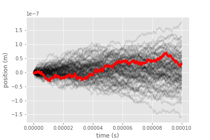
In Week 5 we will use NumPy and matplotlib to analyze an ensemble of Brownian dynamics (random walk) trajectories, which concludes our example on using numpy and matplotlib.
We will then learn about fundamentals of numerical computations, namely how numbers are represented in the computer and what errors one expects in numerical calculations. These two topics are tightly linked and surprisingly, the random walk will show up again in a completely different context.
Week 4 Announcement
In Week 4 we will learn about two fundamental Python packages for scientific computing:
- NumPy, which makes available N-dimensional arrays and functions to work with these arrays.
- matplotlib, a comprehensive library for creating static, animated, and interactive visualizations in Python.
![]()
We will use NumPy arrays as the basic data structure for most of our algorithms and applications, simply because most of Physics can be described as scalar series (e.g., time series), vectors, or tensors. NumPy will enable us to write concise and fast code that operates on these data structures.
Furthermore, all scientific Python packages have adopted the NumPy array as the common data structure so using it makes it easy to work with other packages, too.

matplotlib works seamlessly with NumPy arrays and makes it easy to create 2D plots. It is essential for analyzing the output from our programs. It also has 3D plotting capabilities that we will explore. With some practice, matplotlib can produce publication-ready plots — no more manual graph making in a spread sheet program… Furthermore, because you create graphs by writing Python code, you can fully automate graph creation, which ultimately leads to enhanced productivity and more consistent plots with fewer errors.
Knowing NumPy and matplotlib is absolutely essential when doing scientific programming in Python.
Week 3 Announcement
![]()
In Week 3 we further add to our computational tool belt with a focus on Python itself. After the review of the fundamentals we are now in a position to learn about the power of modularization and code re-use. You’ll also learn some vital tips and tricks for debugging.
Week 2 Announcement
As a computational scientist you want to have a number of tools in your (virtual) tool belt to get your work done. In Week 1 we already learned to use the command line, namely bash.
![]()
In Week 2 we will learn to use the git source code management tool, a distributed version control system (VCS), that is widely used in the open source communities and in industry. A VCS keeps track of multiple files in a project and allows multiple people to work on the same project without overwriting each other’s changes.
![]()
We will also review the Python programming language. Python is widely used in the sciences (and in industry) and provides everything one needs to solve problems in virtually all areas you can think of.
Week 1 Announcement
The plan for this week is to
- install a working environment with Python,
git,bash, and a good coding editor (Atom) on your laptop - learn to use the Unix shell (namely,
bash)
Week 0 Announcement
Hello world!
Welcome to PHY432. We start on 1/14/2025. Bring your laptop to class.
Please check the Canvas (ASU PHY432 Spring 2025) site for additional details.