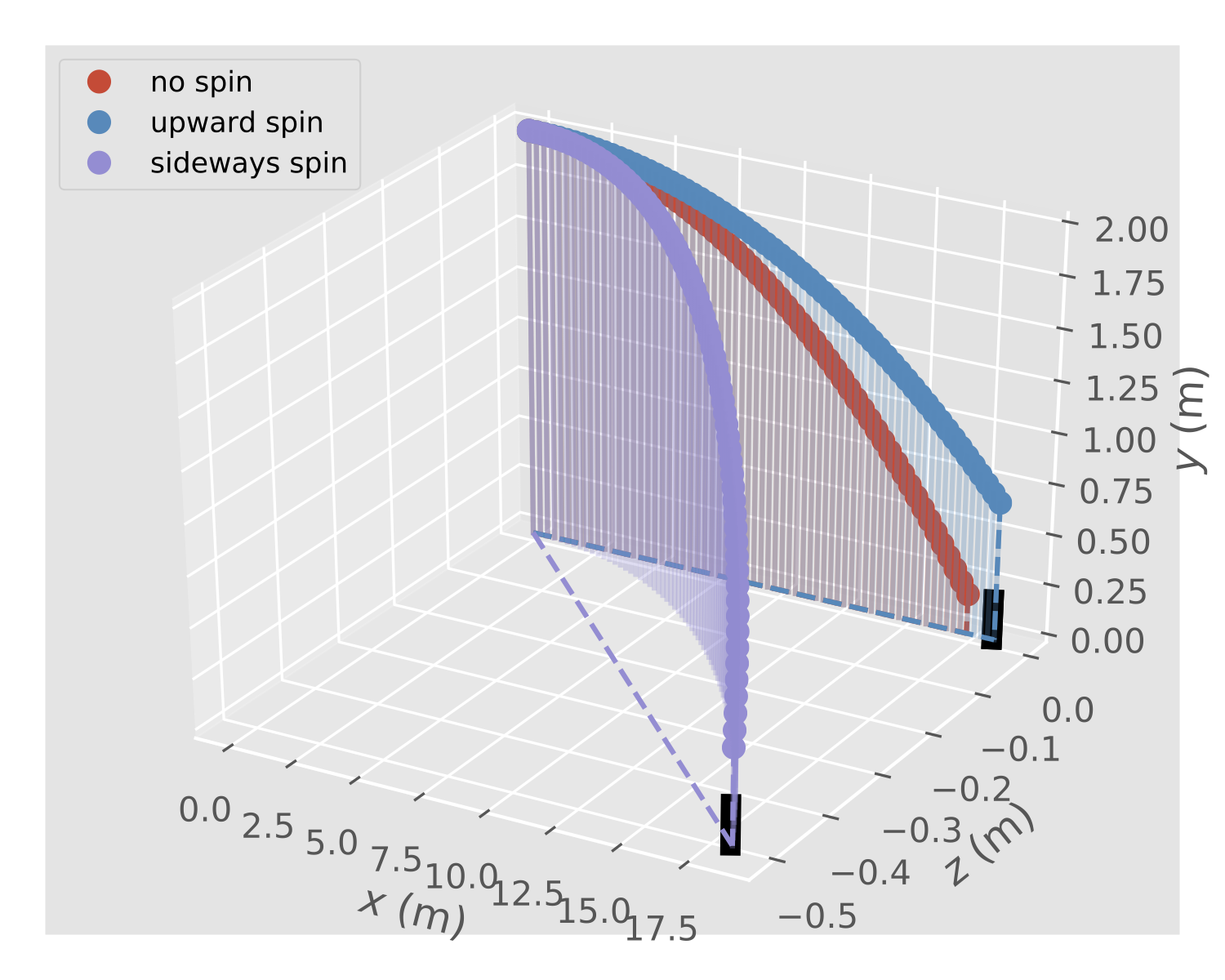
After implementing a number of integrators for ODEs we are now in the position to solve some practical problems:
- movement with air resistance
- realistic movement of a spinning baseball (this lesson)
Baseball physics
The major forces acting on a flying baseball are drag (friction due to air resistance) (see also 11-ODE-baseball.ipynb):
\[\mathbf{F}_2 = -b_2 v \mathbf{v}\]and the Magnus force (when the ball is spinning)
\[\mathbf{F}_M = \alpha \boldsymbol{\omega} \times \mathbf{v}\]where \(\boldsymbol{\omega}\) is the ball’s angular velocity in rad/s (e.g., 200/s for a baseball).
For a sphere the proportionality constant \(\alpha\) can be written
\[\mathbf{F}_M = \frac{1}{2} C_L \rho A \frac{v}{\omega} \boldsymbol{\omega} \times \mathbf{v}\]where \(C_L\) is the lift coefficient, \(\rho\) the air density, \(A\) the ball’s cross section. (Advantage of defining \(C_L\) this way: when spin and velocity are perpendicular, the Magnus force is simply \(F_M = \frac{1}{2} C_L \rho A v^2\).)
\(C_L\) is mainly a function of the spin parameter
\[S = \frac{r\omega}{v}\]with the radius \(r\) of the ball. In general we write
\[\mathbf{F}_M = \frac{1}{2} C_L \frac{\rho A r}{S} \boldsymbol{\omega} \times \mathbf{v}\]For a baseball, experimental data show approximately a power law dependence of \(C_L\) on \(S\)
\[C_L = 0.62 \times S^{0.7}\]The equations of motions are then
\begin{align} \frac{d\mathbf{r}}{dt} &= \mathbf{v}\\
\frac{d\mathbf{v}}{dt} &= -g \hat{\mathbf{e}}_y -\frac{b_2}{m} v \mathbf{v} + \frac{\alpha}{m}\ \boldsymbol{\omega} \times \mathbf{v} \end{align}
(quadratic drag \(-\frac{b_2}{m} v \mathbf{v}\) included.)
The baseball problem was live-coded from scratch during class and the notebook baseball_solution.ipynb1 is a cleaned-up and commented solution. The lesson showed how
- to define the physical problem (obtain trajectory of a baseball with spin and air resistance)
- to derive the underlying equations (Newton’s equations of motions and the forces acting on the ball)
- to adapt an algorithm to solve the equations (use RK4 for integrating the ODEs and express the problem in ODE standard form so that one can use
ode.rk4()) to visualize and discuss the results (plot trajectories and assess the influence of spin)

Resources
- Computational Modelling: Chapter 3
Footnotes
Notebook will be posted after class; in the meantime look at the student notebook. ↩