A large number of problems in physics can be formulated in the language of linear algebra. Not only is quantum mechanics “just” linear algebra over a complex vector space but we encounter repeatedly the case that a large number of equations have to be solved simultaneously in a form that makes them amenable to linear algebra methods.
Basic problems in linear algebra
Coupled linear equations
Given a known \(N \times N\) matrix \(\mathsf{A}\) and an \(N\)-element vector \(\mathbf{b}\), the matrix equation
\begin{gather} \mathsf{A} \mathbf{x} = \mathbf{b} \end{gather}
represents a system of \(N\) coupled linear equations in the \(N\) unknowns \(\mathbf{x} = (x_1, x_2, \dots, x_N)\).
Eigenvalue problem
The matrix equation
\begin{gather} \mathsf{A} \mathbf{x}_i = \lambda_i \mathbf{x}_i \end{gather}
is the eigenvalue problem and a solution provides the eigenvalues \(\lambda_i\) and corresponding eigenvectors \(\mathbf{x}_i\) that satisfy the equation.
Numerical solution
Efficient algorithms exist to solve these problems and we will primarily use the optimized algorithms in the numpy.linalg package:
import numpy.linalgFor most linear algebra work you should be using double precision because diagonalization routines and eigenvalue solvers have problems with nearly singular matrices and the better the machine precision is, the better one can distinguish a nearly singular matrix from a truly singular one.
Problem: One rod, two masses, three strings
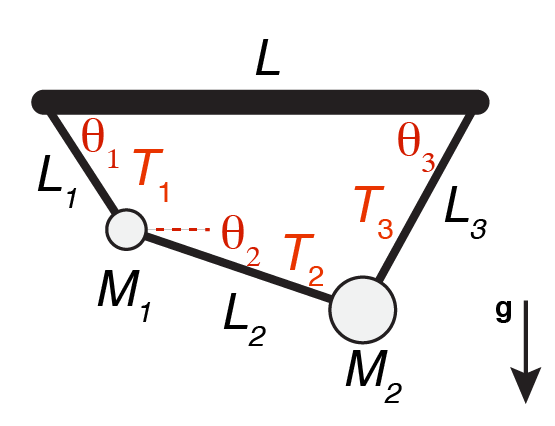
Following Computational Physics (Chapter 6), we want to solve the problem of two masses suspended via three strings from a horizontal rod. The problem with a single mass is trivial and fully determined by the geometry. The problem with two masses is hard but by formulating it as a system of nine coupled non-linear equations in nine unknowns (the three tensions \(T_i\) and, for convenience, we treat \(\sin\theta_i\) and \(\cos\theta_i\) as independent)
\begin{gather} \mathbf{f}(\mathbf{x}) = \mathbf{0} \end{gather}
we can use the generalization of the Newton-Raphson algorithm to \(n\) dimensions to solve it. The generalization involves the computation of the “\(n\)-dimensional derivative”, the Jacobian matrix \(J_{ij} = \frac{\partial f_i}{\partial x_j}\), and the Newton-Raphson method becomes to repeatedly solve the linear matrix problem
\[\mathsf{J}(\mathbf{x}) \mathbf{\Delta x} = -\mathbf{f}(\mathbf{x})\]in order to improve the guess for the solution, \(\mathbf{x}\), with
\[\mathbf{x} \leftarrow \mathbf{x} + \mathbf{\Delta x}.\]Class material
The Jupyter notebook 13_Linear_Algebra.ipynb contains the (life-coded) lecture notes on basic linear algebra. Skeleton code for in-class exercises can be found in 13_Linear_Algebra-students-1.ipynb.1
To get started on the 1 rod/2 masses/3 strings problem work with the notebook 13_String_Problem-Students.ipynb. The full solution can be found in 13_String_Problem.ipynb.
Additional resources:
- Computational Physics: Chapter 6
- 13_linear_algebra notebook (PDF)
- Lecture notes for the 1 rod/2 masses/3 strings problem (PDF) and solution for the problem (PDF)
- Numerical Recipes in C, WH Press, SA Teukolsky, WT Vetterling, BP Flannery. 2nd ed, 2002. Cambridge University Press. Chapter 2.
Footnotes
As usual,
git pullthe resources repository to get a local copy of the notebook. Then copy the notebook into your work directory in order to complete the exercises. ↩