We saw in the Introduction to Python that the Python language has the control and data structures to perform numerical calculations. For instance, a vector \(\mathbf{r} = \left( \begin{array}{c}x\\ y\\ z \end{array} \right)\) denoting the position of a particle could be represented as a Python list r = [x, y, z] and a matrix \(\sigma_{y} = \left( \begin{array}{ccc} 0 & -i \\ i & 0 \end{array} \right)\) as a list of lists sigma_y = [[0, -1j], [1j, 0]].
When it comes to doing numerical work, Python by itself is rather slow. By slow we mean compared to languages like C and Fortran, which benefit from being compiled languages in which a program is preprocessed into machine code by a compiler. Python by contrast is an interpreted language, in which each line in a program is fed to the Python interpreter in sequence, then executed. The flexiblity and ease of use that come with Python come at the cost of pure performance.
![]()
However, though Python code itself may be slow, Python can be used to run code that is written in a compiled language and already compiled. We will use a library (a.k.a., a Python package) that does exactly this underneath the hood to get fast performance for numerical operations on arrays: We load the NumPy package:
import numpyWe will learn the basics of NumPy.
Table of contents
Class material
The class will be live-coded in a Jupyter notebook. The annotated notebook is available as 06-intro-numpy.ipynb.
You can load the notebook yourself: first update your local PHY432-resources repository1
cd ~/PHY432-resources
git pull
Copy the notebooks to your work directory
cd ~/PHY432
cp -R ~/PHY432-resources/06_numpy .
cd 06_numpy
and launch the Jupyter notebook interface in your web browser2:
jupyter notebook- Select the notebooks live/06-intro-numpy-LIVE.ipynb from the list if you want to work along with your instructor.
- Select the notebooks 06-intro-numpy.ipynb from the list for the complete notebook (e.g., when reviewing).
See How to use the notebook for basic notebook commands.
numpy key concepts
The NumPy package is an essential Python package that makes scientific and numerical work with Python possible. It primarily provides the array data structure as the ndarray class. (“N-dimensional array”).
NumPy arrays are of fixed data type and fixed size. They support
- arbitrary dimensions
- fast indexing and slicing
- fast element-wise array arithmetic with broadcasting
- fast element-wise universal functions (ufuncs)
Load NumPy with
import numpy as np
Example array:
>>> a = np.arange(24).reshape(6, 4)
gives
array([[ 0,  1,  2,  3],
       [ 4,  5,  6,  7],
       [ 8,  9, 10, 11],
       [12, 13, 14, 15],
       [16, 17, 18, 19],
       [20, 21, 22, 23]])
This is an array with two dimensions (one needs two indices to find an element). The dimensions are called axes in numpy (axis 0 and axis 1). The shape of the array is (6, 4) because there are 6 elements along axis 0 and 4 elements along axis 1. numpy arrays can have arbitrary dimensions and shape (only limited by the computer memory).
Array indexing/slicing
Indexing and slicing looks similar to how we accessed elements and slices of lists but generalizes nicely to higher dimensions (and is much faster in NumPy).
Multidimensional indexing:
>>> a[5, 3]
23
Multidimensional slicing:
>>> a[1:3]
array([[ 4,  5,  6,  7],
       [ 8,  9, 10, 11]])

>>> a[1:3, :-2]
array([[4, 5],
       [8, 9]])
Advanced slicing
Arrays are more versatile than lists. We can slice them with other arrays and efficiently read out any parts of the array in a very succinct (and fast) manner.
>>> a[[0, 2, 1]]
array([[ 0,  1,  2,  3],
       [ 8,  9, 10, 11],
       [ 4,  5,  6,  7]])
Boolean arrays:
>>> even = (a % 2 == 0)
>>> even
array([[ True, False,  True, False],
       [ True, False,  True, False],
       [ True, False,  True, False],
       [ True, False,  True, False],
       [ True, False,  True, False],
       [ True, False,  True, False]])
can be used for pulling out elements for which the indexing array is True
>>> a[even]
array([ 0,  2,  4,  6,  8, 10, 12, 14, 16, 18, 20, 22])
or for setting specific elements to one value
>>> b = a.copy()
>>> b[even] = -1
>>> b
array([[-1,  1, -1,  3],
       [-1,  5, -1,  7],
       [-1,  9, -1, 11],
       [-1, 13, -1, 15],
       [-1, 17, -1, 19],
       [-1, 21, -1, 23]])
Array arithmetic
Arrays support element-wise arithmetical operations. Understanding this seemingly simple concept is key for making best use of arrays.
Scalar multiplication
>>> 2 * a
array([[ 0,  2,  4,  6],
       [ 8, 10, 12, 14],
       [16, 18, 20, 22],
       [24, 26, 28, 30],
       [32, 34, 36, 38],
       [40, 42, 44, 46]])
Element wise operations
>>> a + b
array([[-1,  2,  1,  6],
       [ 3, 10,  5, 14],
       [ 7, 18,  9, 22],
       [11, 26, 13, 30],
       [15, 34, 17, 38],
       [19, 42, 21, 46]])
It leads to “thinking in arrays” (below) for creating highly performant code in Python that nevertheless looks almost like the mathematical equations that one started from.
Thinking in arrays
Once you learn to “think in arrays” you can use arrays and array arithmetic with array slices to create code that is much faster than standard Python code with loops or list comprehensions make your code much more readable (and thus more easily to understand and to debug).
For example, calculate the midpoints m \(m_i = \frac{1}{2}(e_i + e_{i+1}), 0 \le i < N-1\) from the edges \(e_i, 0 \le i < N\) in array e
>>> e = np.array([1, 2, 3, 4, 5])
>>> m = 0.5 * (e[:-1] + e[1:])
>>> m
array([1.5, 2.5, 3.5, 4.5])
Array methods
The ndarray object has a plethora of methods and attributes.
shape and dimensions
>>> a.shape
(6, 4)
>>> a.ndim
2
Transposition
>>> a.transpose()
array([[ 0,  4,  8, 12, 16, 20],
       [ 1,  5,  9, 13, 17, 21],
       [ 2,  6, 10, 14, 18, 22],
       [ 3,  7, 11, 15, 19, 23]])
>>> a.transpose().shape
(4, 6)
Aggregation, e.g., the arithmetic mean
>>> a.mean()
11.5
Aggregation can be performed along one axis:
>>> a.mean(axis=1)
array([ 1.5,  5.5,  9.5, 13.5, 17.5, 21.5])

>>> a.mean(axis=1).shape
(6,)
See the documentation for all methods or use introspection in ipython (<TAB> completion) to learn more.
Broadcasting
In order to make “thinking in arrays” work seamlessly, it is necessary to have a mechanism to perform arithmetic with arrays of different dimensions (shapes) and arrays and scalars (numbers). In NumPy, broadcasting describes how numpy treats operations between arrays of different shapes. Basically, the smaller array is “expanded” or “stretched” or “replicated” in one axis so that its shape becomes compatible with the bigger array.
This makes it possible to avoid writing explicit loops, which generally means faster and more readable code.
From the SciPy Lecture Notes: NumPy: creating and manipulating numerical data:
- Basic operations on
numpyarrays (addition, etc.) are element-wise - This works on arrays of the same size.
- Nevertheless, It’s also possible to do operations on arrays of different sizes if NumPy can transform these arrays so that they all have the same size: this conversion is called broadcasting
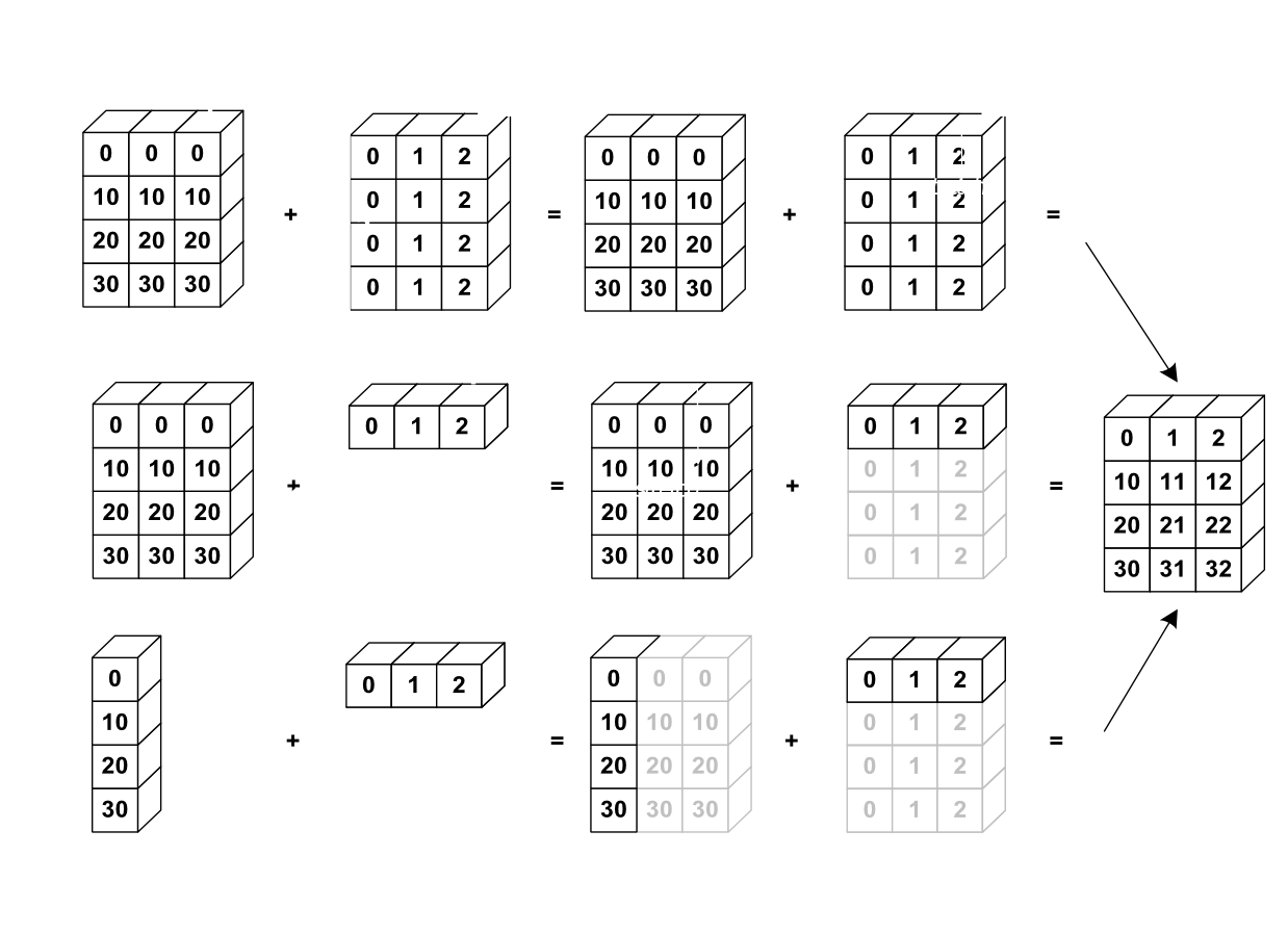 numpy broadcasting: the smaller array is “expanded” to fit the larger array so that element-wise operations can be performed. (Image from https://scipy-lectures.org/intro/numpy/operations.html by Emmanuelle Gouillart, Didrik Pinte, Gaël Varoquaux, and Pauli Virtanen, used under CC-by 4.0 License).
There’s also a long article on Array Broadcasting in NumPy in the numpy docs.
It takes a while to wrap one’s head around broadcasting. It is very useful to try it out in the Python interpreter or in a notebook and just play with simple arrays. When you develop code, prototype your array arithmetic interactively (and look at the shape of your intermediate arrays). You will be rewarded with elegant and fast code.
Universal functions (ufuncs)
The final missing functionality to make arrays work is a way to work with functions and arrays without needing to use loops. ufuncs are functions that operate on ndarrays in an element-wise fashion and return an array of the same shape as the input array. For example:
import numpy as np
import matplotlib.pyplot as plt

X = np.linspace(-10, 10, 200)
Y = np.sin(X)

plt.plot(X. Y)
Note that all the calculations of \(sin(x)\) are performed in the simple line Y = np.sin(X) where the ufunc np.sin operates on the array X.
Resources
- NumPy Quickstart Tutorial
- Jay Alammar’s A Visual Intro to NumPy and Data Representation
- Jake VanderPlas Python Data Science Handbook, Chapter Introduction to NumPy
- Software Carpentry Analysing data with numpy and matplotlib
- Software Carpentry Advanced NumPy
SciPy Lectures 1.3. NumPy: creating and manipulating numerical data by Emmanuelle Gouillart, Didrik Pinte, Gaël Varoquaux, and Pauli Virtanen.
(The SciPy lectures are an outstanding learning resource and if you only had one place on the internet to learn scientific programming in Python then this would be it!)
- Harris, C.R., Millman, K.J., van der Walt, S.J. et al. Array programming with NumPy. Nature 585, 357-362 (2020). DOI: 10.1038/s41586-020-2649-2.
Footnotes
If you have not set up your PHY432-resources repository then revisit PHY432 Workflow. ↩
If you have problems launching the notebook interface on Mac OS X, try
jupyter notebook --ip=127.0.0.1If problems persist, search the internet for the error message and ask for help. ↩